
300 House Inventions
list
and Video

Mostly by White men
The Demographics of Inventors in the Historical United States
January 10, 2016
www.law.Northwestern.edu/research-faculty/clbe/events/innovation/documents/Sarada_patent_grantees_Dec_2015.pdf
pdf


Abstract
Who invents? This is a central question to understanding possible barriers to entry in the innovation process. To address it, we match the Annual Report of the Commissioner of Patents from 1870 to 1940 to the corresponding U.S. Federal Population Censuses. This matching procedure provides a rich set of demographic information on a comprehensive set of inventors. We first document that patentees over this seventy year period are more likely to be older, white, male and to be living in a state other than the one in which they were born. Surprisingly, these patterns are very persistent over space and time though the fraction of women appears to rise slightly. We then attempt to correlate the demographics of patentees with county-level economic and demographic characteristics. Beyond the most obvious such as the number of a particular group in that county, very little explains differences in the demographics of inventors across counties. This suggest that most barriers to entry are persistent over time and very little across space.
We thank the Minnesota Population Center for making available the 100% Census files, the Kauffman Foundation for financial support, and Siha Lee for excellent research assistance. We also thank audiences at the Iowa Macro Workshop, Yale Economic History, Wisconsin Agricultural Economics Department, and Kauffman Foundation.
Introduction
Invention is at the root of economic growth. While economists have a rich understanding of the economics of innovation at a theoretical level, much less is known about the individuals who actually generate these innovations. For example, where do inventors come from? What drives marginalized groups to undertake these activities? What institutional features encourage (or discourage) such activity? Understanding these demographic and institutional differences is essential for fostering broad participation in the creative process, which is, in turn, crucial for the process of growth.
To shed light on this process, we build a comprehensive dataset by matching people who were granted a patent in the years 1870, 1880, 1900, 1910, 1920, 1930, and 1940 to the corresponding decennial US Population Census. This matching procedure delivers a variety of demographic information on these individuals such as age, race, gender, and family structure. While others have constructed limited samples of historical inventors, our matched dataset provides a richer view of the demographics of historical patentees, covering the entire universe of US patents over a period of 70 years.
First, we find that across our this 70 year period, inventors are demographically quite different from the general population. This is true in some obvious ways including that fact that patentees are more likely to be white and male. It is also true in less obvious ways including the fact that they tend be older, and to be living in a different state than that of their birth. For the most part, these patterns are stable across our seventy year period, with some variation in these trends across time. In particular, there is a high degree of persistence in the extent to which older individuals and people not living in their state of birth are overrepresented in the patentee population across time. On the other hand, over our timeframe, women go from comprising 2% to comprising 15% of patentees while making up about 50% of the general population. Non-whites however, are consistently underrepresented between 1870 and 1920 but experience a striking sea change beyond that to become overrepresented past 1930. This increased minority representation however, does not come from blacks who are always underrepresented, making up 6% of the patenting population across the seventy years, while comprising between 10 and 13% of the general population over that same timeframe. Instead, the data suggests that non-black minority populations (possibly Asians and Hispanics) are the ones to drive this shift in minority patenting rates.
We find it useful to put these patterns for women and non-whites in perspective by highlighting the incredible degree of persistence in the demographics of inventors from the middle of the 19th century all the way up to the present given the ostensible increased access to civil rights, education and labor force participation afforded to both groups over the past 140 years. Simply put, women and blacks to this day account for a disproportionately low fraction of inventive activity. Ding et al. (2006) show, using recent data from the life sciences, that 5.65% of women scientists patented at all (as compared to 13% of male scientists) to hold only about 6% of filed patents. Additionally, Ashcraft and Breitzman (2007) find that in the IT sector only 9% of patents involve any female patentees. When they account for the fact that most patents involving one woman also involve multiple males, this brings the percentage down substantially, to about 5%. While some of these studies such as Ding et al. (2006) and Frietsch et al. (2009) find declining gender gaps, this catchup is slower than female engagement in other comparable parts of society such PhD education in Science and Engineering (Jung and Ejermo, 2014), and is far from common across countries and types of inventive activities (patenting vs. academic publishing). More importantly, all studies still find large gender gaps. Similarly, the participation of blacks in patenting activity today remains dismal (Cook, 2004).
It is interesting to ponder what explains the differences in the increased participation of these marginalized groups across different “knowledge intensive” activities. Inventive activity as measured by patents granted or academic papers published seems to fall much closer to finance, which has had a small increase in participation by these groups e.g. Bertrand et al. (2010) on women. While at the same time, these groups have rapidly increased their representation in the medical profession (Hsieh et al., 2013) where women, for example, now almost outnumber men in medical school. Hunt et al. (2012) argue, at least, that lower patenting rates for women are not due mainly to low rates of science and engineering degrees but rather, these degrees do not appear to translate into representation in engineering or R&D jobs -presumably where a substantial amount of patenting occurs.
Finally, putting the age patterns in a modern context, we find some differences. In particular, along a number of measures, it seems that the age of innovators has been increasing over the last 50 years. For example, the age of first time NIH grant recipients has steadily increased from 37 in 1980 to 42 in 2008 (Kaiser, 2008). Jones (2009) shows that the age of first invention has been increasing between 1985 and 2000. He attributes this trend, at least in part, to the increased time necessary to acquire the human capital to invent. On this point, Jones (2010) documents that the average doctoral age of Nobel Prize winners in the 20th century has been increasing as well. However, since 2000, the average age of all inventors and first-time inventors has been declining quite rapidly from a peak of just over 46 in 1997 to 43.4 in 2007 as noted by Jung and Ejermo (2014). So perhaps the patterns observed by Jones between the mid 1980s to 2000 were simply transitory and the ages of inventors are returning to something like they were back in 1900 when patentees were just over 15% older than the whole US population translating to an average age of 40.3.
We also find that inventors are much less likely to be living in the state of their birth. We cannot identify (at this point) how long a particular inventor has been living in a particular location before patenting. So right now this fact is simply suggestive that these people are moving to areas with greater opportunities. This pattern echoes a sequence of papers by (Kerr, 2008; Kerr and Lincoln, 2010; Kerr, 2010; Foley and Kerr, 2013) about the large contribution of immigrants to innovation in 20th century America. We can document in our 1900 data that individuals with immigrant parents flourish in inventive activity. These are rather striking when contrasted to the obstacles faced by women, blacks and certain types of immigrants -in particular the those coming to the US during the Mass Migration (Abramitzky et al., 2012).
After documenting these time patterns, we estimate the relationship between county-level economic and demographic factors and the demographics of patentees. We find, not surprisingly, that counties with more women (resp. blacks or an older population) tend to have more women (resp. black or older) patentees, but the elasticity is much smaller than 1. So the process by which a particular type of patentee is generated is not simply a random draw from the underlying county population. Other characteristics of the county such as population and the fraction of employment in manufacturing have inconsistent effects across demographic groups and across specifications for the same demographic group. We conclude from this that, at least the most obvious, observable county-characteristics do not explain the differences in the representation of various demographic groups in patenting activity. 1
One obvious limitation of this work and all work using patents is the extent to which patents really capture the totality of inventive activity in terms of quality and quantity. It may be the case that marginalized populations are equally likely to invent, but simply do not patent -especially if they lack the resources necessary to file and enforce their patent. For the 19th century, (Cook, 2014) argues that blacks often patented under the white names of their lawyers. Thursby and Thursby (2005) find in their sample of scientists in the late 20th century that, while publication differs slightly across genders, women are much less likely to disclose a potentially commercializable invention (though Cook and Kongcharoen (2010) find similar rates of patent assignment for women and blacks relative to the whole universe of patents granted between 2001 and 2008). We would argue that even in the case where patenting is in some way a flawed measure of innovative activity
Of course, there are many other possible local characteristics or institutions that could effect these demographics that we do no consider. For example, (Cook, 2014) studied the relationship between lynching and black patenting. Another possibility is the existence of a Historically Black College or University.
(as surely is any single measure), differences in patenting rates across demographic groups are still informative as to the perceived returns to patenting by demographic group.
Our work is related to the series of papers by Ken Sokoloff and co-authors (Sokoloff, 1988; Sokoloff and Khan, 1990; Khan and Sokoloff, 1993; Lamoreaux and Sokoloff, 2005) that studied patenting rates in 19th century America building on the pioneering work of Schmookler (1957). In his original 1988 work, he constructed a random sample of patent holders from the same primary source covering from 1790 to 1846. He documented some broad patterns such as the pro-cyclicality of patenting and a relationship with the growth of markets during industrialization. Later work extended these data to address questions of entrepreneurship as well as some basic facts about the demographics of the inventors. Perhaps most closely related is the work by Lamoreaux and Sokoloff (2005), who drew three random cross-sectional samples (totaling about 6,600 patents) from the same Annual Reports of the Commissioner of Patents for the years 1870-71, 1890-91, and 1910
11. For each patent in the samples, they recorded a brief description of the invention, the name and location of the patentee(s), and the names and locations of any assignees granted rights to the invention before the date the patent was issued. In addition, they constructed a longitudinal dataset selecting from the three cross-sectional samples all (561) inventors whose last names began with the letter “B.” For this set, they then collect information from Patent Gazettes and from the Annual Reports of the Commissioner of Patents for all of the (6057) patents obtained by these patentees for the twenty-five years before and after they appeared in one of our samples. Finally, they collected similar information for patents granted in selected years to “great inventors” as defined by being in the Dictionary of American Biography and born between 1820 and 1885. While this latter source provides detailed descriptive information, it is limited to a selected group of the “great inventors.” Our innovation is in the number of innovators we obtain demographic information on which allows us to document and comment on the more general trends in the American creative process.2
2 Data
We offer a short discussion here of our procedure for building this dataset. More details are available in the appendices. We followed a three step process: (1) obtaining machine readable versions of
2
In addition, Cook (2011) constructed a sample of black inventors between 1870 and 1930 based on biographies from the NAACP from the 19th century.
the Annual Report of the Patent Commissioners; (2) parsing those reports into fixed format files; and (3) matching those files against the corresponding Population Census. Issues can arise at all three of these steps that might bias the final sample.
First, we obtained a machine readable version of the Annual Report of the Commissioner of Patents from archive.org for the Census years. These reports include the names of patent grantees, the town and state in which they lived, the invention name, and the type of intellectual property including utility, design, and plant patents. They also contain modifications to earlier patent applications in the form of disclaimers and, in most years, a list of registered trademarks and labels. These volumes were digitized by Google, and while the transfer to digital format appears to have been good, it is not perfect. In particular, the photocopied volumes have a particularly high number of unreadable pages in 1920 and 1930, the two years with the lowest parse rate. In addition, the format in which information about each patent is recorded is not consistent over years, with some years being more amenable to parsing. This second issue is particularly pernicious in 1930 and 1940, resulting in very low match rates. Consequently, results for 1930 and 1940 should be considered extremely preliminary. We are addressing these issues in future iterations of the parsing algorithm. In spite of these difficulties, we believe our parsed results are representative of the overall population of patentees. In Appendix A, we provide some evidence for this claim using another dataset of patentees collected by Jim Shaw. Overall, as noted in Table 1, the parser is able to extract between 36 and 72% of the patents granted each census year between 1870 and 1920 comparing our totals to the totals listed in the Annual Report.
The next step is to match these names to the 100% sample of the decennial Census of Population provided by the Minnesota Population Center. The Census data offer basic demographic information such as race, age, gender, as well as information on birthplace for the individual and the individual’s parents consistently across all the years.3 We compare the demographics of the patentees to the underlying demographics of the county-level population from which they are drawn. We complement the population census data with information from the NHGIS, which has created county-level datasets drawn from the the manufacturing and agricultural censuses. These latter economic variables serve as explanatory variables in the regressions that we estimate.
These are of course not all of the questions asked by the Census in any given year. Unfortunately, not all the variables have been transcribed though some specific ones such as literacy have been for particular years. That said, the 1940 file has much more detailed information on educational outcomes and income.
Matching statistics for each year are also reported in Table 1. For each year from 1870 to 1920, we find a match for 52-65.5% of the parsed patents. In terms of the total number of granted patents, including those that could not be parsed, we match 20-50% for 1870 to 1920.4 Our match rates are higher than those reported in Long and Ferrie (2013) and Abramitzky et al. (2012) of around 30%. We believe this reflects the fact that we match on only a few identifying characteristics.
At the same time, the fact that we search for people in very narrow geographic regions mitigates the problem of multiple matches. Recall that each patentee may receive multiple possible matches from the census data, and, in fact, the same person in the census may match to the same patentee. There is no requirement that the matching be “injective.” Still for 1870, 1880, and 1910, about 85% of the patentees were uniquely matched. Not surprisingly, the fraction of uniquely matched patents decreases in 1920, 1930, and 1940 as population grows. The number of potential matches per patent increases from an average of 2.79 possible matches in 1870 to almost 30 possible matches in 1940. We also report the number of “perfect” matches, which are matches in which all of the characters in the last name, first name, and town of an individual in the census match exactly with an inventor in the patent report.
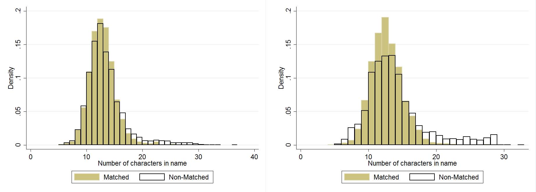
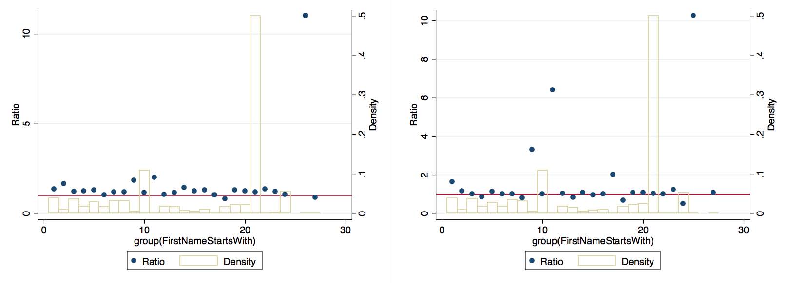
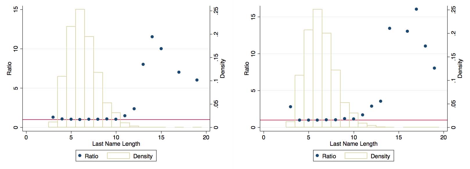
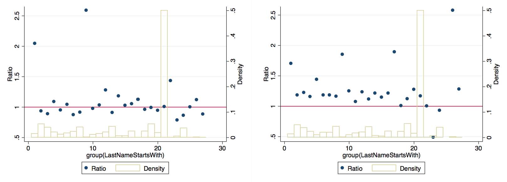
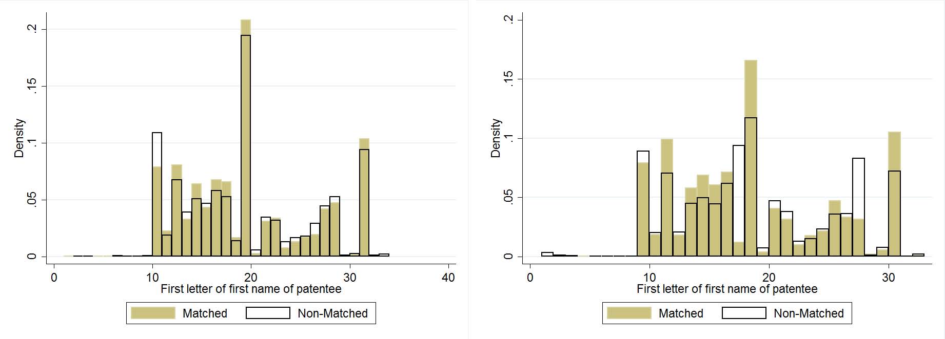
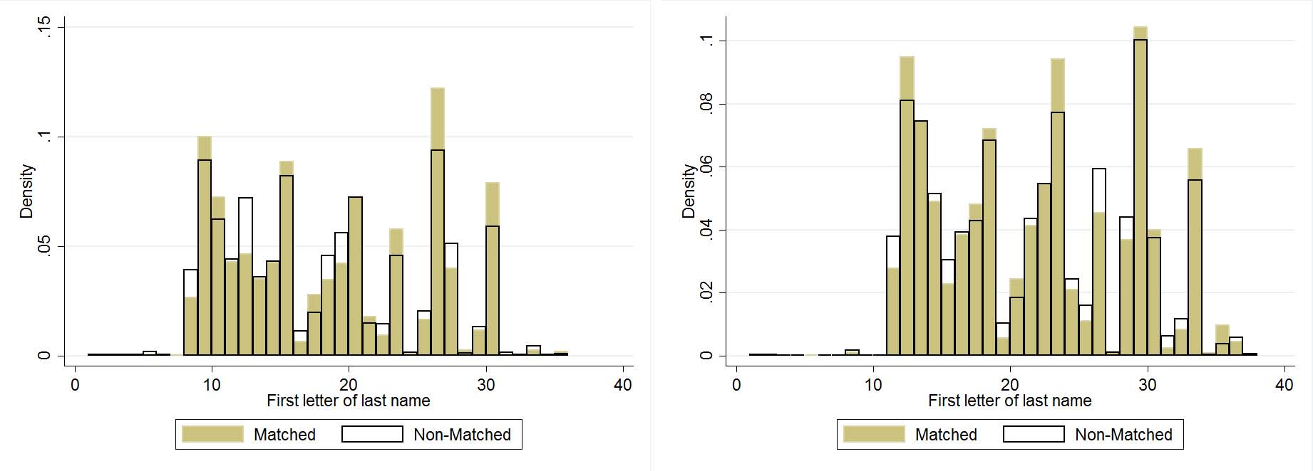
A crucial question is to what extent the matched sample is representative of the whole sample. This is of course impossible to demonstrate for unobservables (by definition), but we can show that along a number of observable dimensions, the matched sample looks similar to the non-matched sample. Figure 8 displays this comparison for 3 different characteristics for the census years of 1880 and 1920: first letter of first name, first letter of last name, and number of characters in name. Results for the other census years are very similar. There are any number of reasons the matched sample could differ from the non-matched sample. For example, given how the matching algorithm compares strings, the length of the string may make it easier (or more difficult) to declare a match. However, as is evidenced in the panel (c), there is no meaningful difference here in most years. There is likewise negligible difference in first letters of first and last names. This gives us some confidence that our matching procedure is not biasing the sample towards particular types of patentees.
The current issue with 1930 and 1940 is that our match rates are much lower at around 10% of the parsed patents and 5-7% of the full population of granted patents. We believe this low match rate is due to parsing errors in these years which produces impossible-to-match town names. We are working to correct this issues in future versions of the paper.
3 Results
3.1 Trends in the Demographics of Patentees
Over the whole 70 year time frame, patentees are on average 40 years old as compared to the population average of 37 conditional on individuals being at least 10 years old. Across our sample,
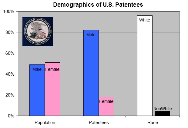
82% of patentees are male as compared to 50% in the general population. 96% of patentees are white and 66% are cross state immigrants. We find what we would consider “relatively high” rates of patenting by two marginalized groups: (1) women and (2) blacks. Though still much lower than their proportions in the population, the rate of female patenting ranges between 10 and 24% while the rate of black patenting runs between 3 and 10%. At least for blacks, there is some reason to believe that these numbers are an underestimate as suggested by Cook (2014). She argues that blacks tended not to file under their own names because of worries about how their patent would be viewed.5
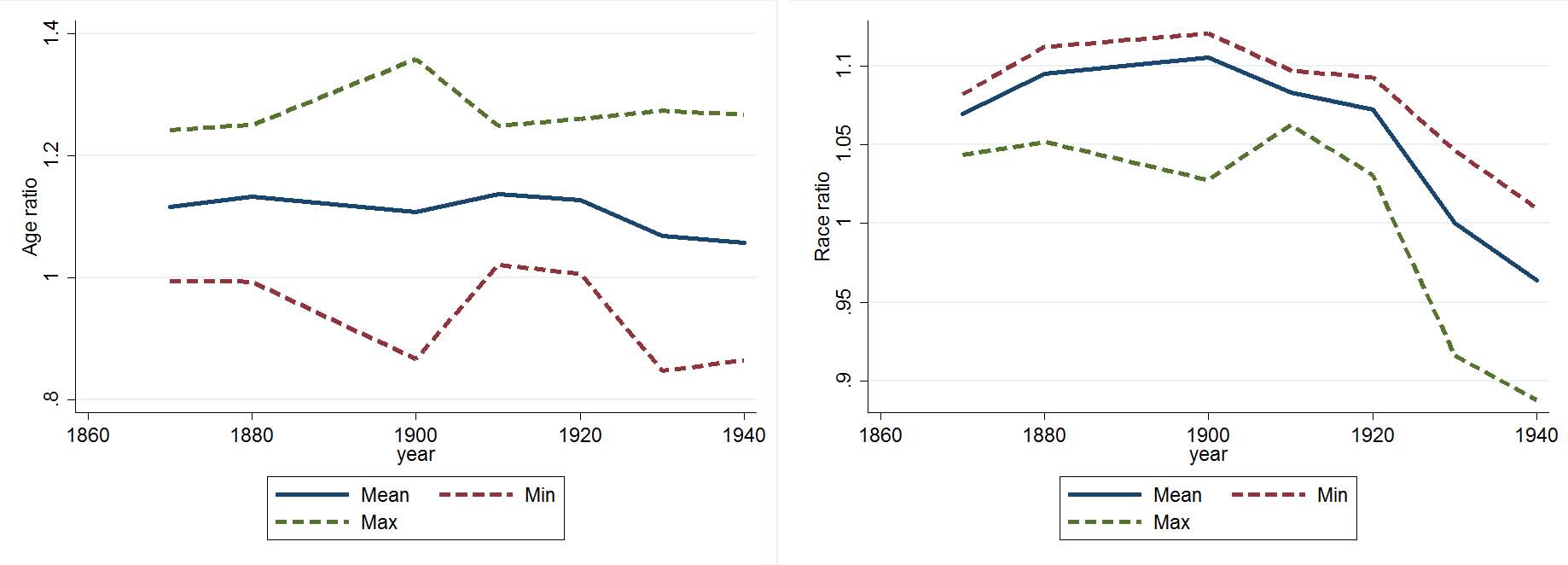
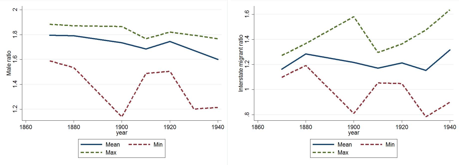
Next, in Figure 1, we document some simple time series patterns of the demographics of patentees relative to the general US population. We plot the following lines. Let X be some demographic variable (age, sex, race, migration status) and let i = 1....N index patents, then we calculate
1
1. XU = i maxj Xij
N
1
2. XL = Ni minj Xij
11 mi
3. XM = N imi j=1 Xij
where j =1...mi indexes possible matches for patentee i. The first two can be thought of as “worst case” bounds in that the “true” average must lie between them. The third measure simply averages across patentees and their potential matches.6 We then plot these statistics normalized by the average value of the demographic variable in the county of the patentee’s residence. So a value of 1 means that the demographics of inventors in a particular county are representative of the county population as a whole.
5
At the same time, there are questions about what legal recourse blacks would have in this case if the white person filing the patent decided to use the patent in some way contrary to the black inventor’s intentions.
6
Note that we could have also plotted the time series based on our best match for each patentee or for only the set of patentees that have a unique match. We chose these three series to maximize the number of patentees included in constructing the time series patterns.
In Panel (a) we show that consistently over this time period the average age of patentees was about 15% higher than the population as a whole. Recall that this is after eliminating everyone under 10 years of age. This pattern fits more recent studies as well such as that of Jung and Ejermo (2014), but contradicts that of jones:2009a, who seems to suggest that the age of inventors should be increasing faster than that of the reference population. Note that the worst case bounds, while showing different levels of average age (the lower bound suggests patentees are younger ), does not show drastically different trends over time. We take the relative stability as the most salient and striking feature particularly in light of the changing composition of industry and areas of greatest inventive progress.
Panel (b) shows that relative to their representation in the population, whites are overrepresented among patentees between 1870 and 1920. However, between 1930 and 1940, this pattern is reversed where non-white patentees become the more heavily represented group. We find the last two observations rather anomalous. So we focus on the first 50 years and again what strikes us is the relative stability of black patenting rates. This is in the face of the imposition of Jim Crow laws after the end of Reconstruction in 1877. These laws severely restricted the political rights of black in many southern states and set up a separate (and underfunded) school system for blacks.
Panel (c) shows that female patentees are severely underrepresented throughout our timeframe, representing between 2 and 15% of patentees while comprising about 50% of the population. This disproportionate underrepresentation monotonically declines between 1870 and 1910, and then at a (slightly) faster rate from 1920 onward -coinciding with the women’s rights movement. While this brings the gender composition of patentees slightly closer to that in the population, the divergence remains large. The worst case bounds show broadly similar patterns here though the drop in in the lower bound is exaggerated. Whether the relationship between increases in formal political and economic rights and patenting representation of women is more than spurious demands closer scrutiny. Note however that all of this increase precedes the large increases in female workforce participation dating to after the second World War. It is interesting to set that casual correlation against the limited change in the representation of blacks in patenting as the Jim Crow system of disenfranchisement and segregation intensifies over this period.
Our final broad time series pattern in panel (d) shows that patentees are more likely than the overall population to reside in a state other than their birth state. While there are some fluctuations in the overrepresentation of migrants amongst patentees, the overall pattern is relatively stable across time. Perhaps this can be explained by the differences in demographics presented in the other three panels (or simply state of birth). Still we find it suggestive of moving to opportunities that patentees tend to be living outside their state of birth. Understanding what drives this location decision is a key question for future research. We would note here that the worst case bounds suggest differ patterns with the representation of migrants increasing over time for the upper bound and decreasing over time for the lower bound.
Turning to the nativity of the inventor’s parents, we find about 52% of inventors have a native born father and about 54% have a native born mother. Given the high rates of homogamy, the fraction that had at least one native born parent was 53%. The fraction of inventors living in their birth state and having native fathers and mothers are much lower than the rate for the overall population, suggesting that inventors are more mobile and that immigrants and children of immigrants play a disproportionately large role in innovation. This is in line with the findings in the papers by Kerr (2008); Kerr and Lincoln (2010) that use ethnic names to estimate the impact of immigrant and early generation inventors during more recent years.
3.2 Patenting rates based on first names
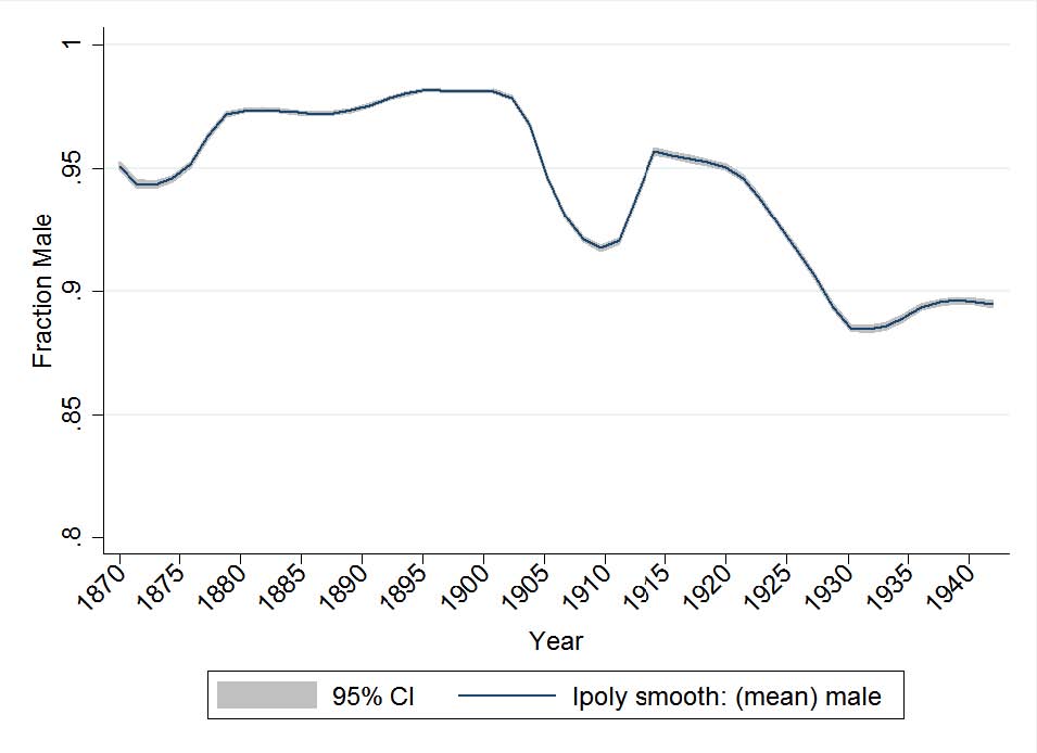
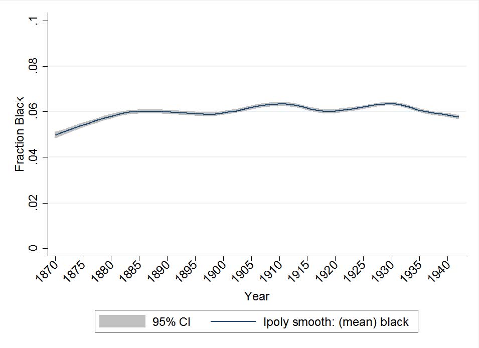
As a check on the quality of the matching and as a way to get a more complete time series picture, we offer a second method for inferring the gender and race of patentees for all years not just Census years. In particular, we use the observed probability a person is black (male) as a function of the first name of the person. This of course could be extended to other observable characteristics such as state of residence or last name. For example, Cook et al. (2013) have done this historically for black names and identified a set of “distinctively black names.” It has been used in a number of papers on patenting as well such as Jung and Ejermo (2014) to infer gender, Jones (2009) to infer age, and Celik (2015) to infer income. One upshot of this approach is that we can use the first name probabilities based on the Census to calculate the average fraction of black and female inventors for any year of the Annual Report. We do not have to restrict attention to only Census years in calculating this probability. Concretely, using the 100% Census dataset, for each first name η, we calculate pη = P r(Black|η), similarly for women. Then, for patentee i with name ηi in a given patentee list, we impute the probability being black using pηi . Then our estimate of the fraction of
black inventors is given by 1 #ηpη
N
η where #η is the number of patentees with name η. This procedure is basically a split-sample IV procedure (Angrist and Krueger, 1992).7
Figure 2 shows the results based on this procedure for gender and race. We find broadly similar patterns to those from our “exact” matching routine. In particular, there is a remarkable amount of stability in the prevalence of these groups in patenting. At the same time, there are differences. For one, the change in black patenting rates is much smaller to non-existent with this procedure. Second, it is also quite clear that the overall increase in female patenting takes place after 1900 in a more or less secular fashion (though this only constitutes a few percentage point increase).8
3.3 Ages of Marginalized Groups
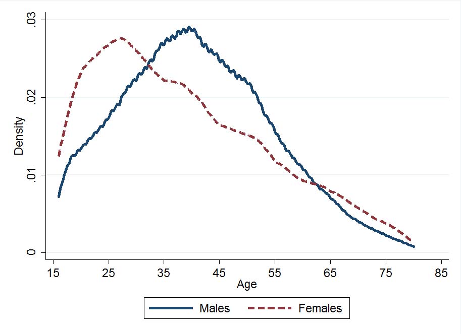
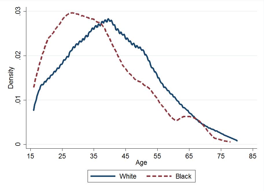
We now compare the age distributions of females relative to males and blacks relative to whites. Figure 3 shows a striking difference in the age distributions of female patentees and black patentees as compared to all other patentees. The median female patentee is about 10 years younger than the median male patentee. Similarly, the median black patentee is 10 years younger than the median white patentee. While the graphs displayed include data from the entire sample, these findings hold in every year. One possible explanation is that women and blacks face greater hurdles in accessing education and high skill employment. As such, they start inventing earlier rather than doing so after acquiring more formal human capital. An alternate explanation is that females and blacks invent just once, either due to factors precluding them for repeat invention or because they are not employed by larger firms that facilitate careers in invention. In future work, we plan to track inventors over their entire life cycle, which will allow us to more directly observe how patenting behavior changes with age for different demographic groups. In the case of women, it could also simply be that they dropped out of the workforce by their early 20s to start a family, which spells the end of their possible contribution. It would be interesting to examine how this pattern changes as women enter and stay in the workforce in much greater numbers after WWII.
7
We could apply a similar procedure to inferring ages as well 8Note that we are still not able to code all names in the Annual Report since they are not in the Census. This is due to mistakes in the names and was part of the motivation for moving to the fuzzy matching procedure we employ.
3.4 Geographic Patterns
We now consider some state and county-level patterns in patenting. This returns to earlier work by Sokoloff (1988) on the distribution of patenting in the US and more recent work by Perlman (2015) examining the relationship between patenting and transportation networks.
3.4.1 State-level
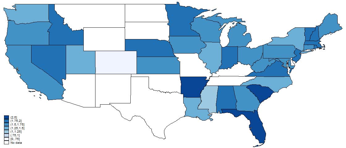
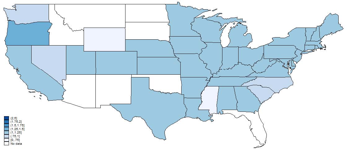
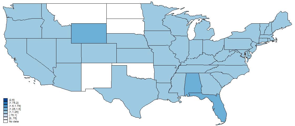
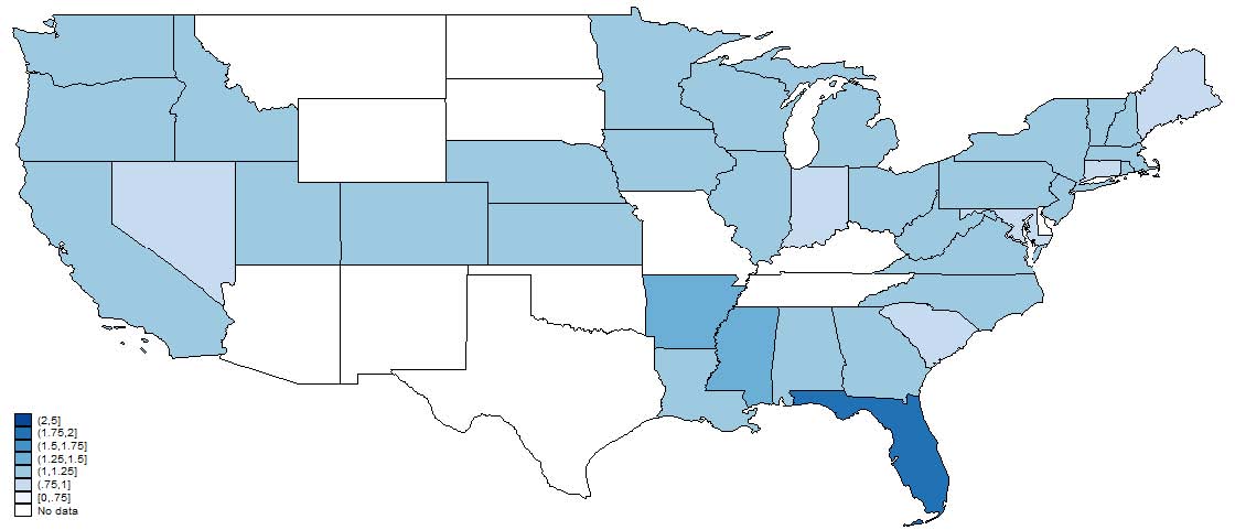
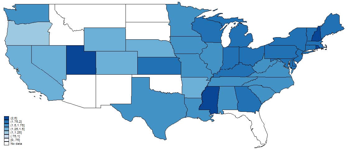
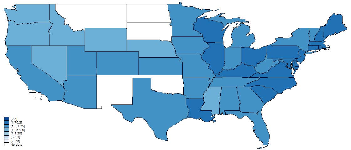
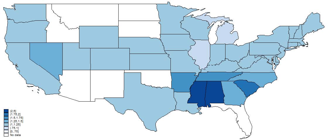
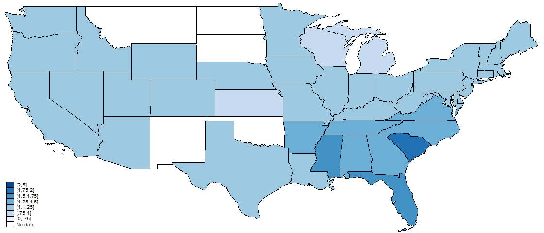
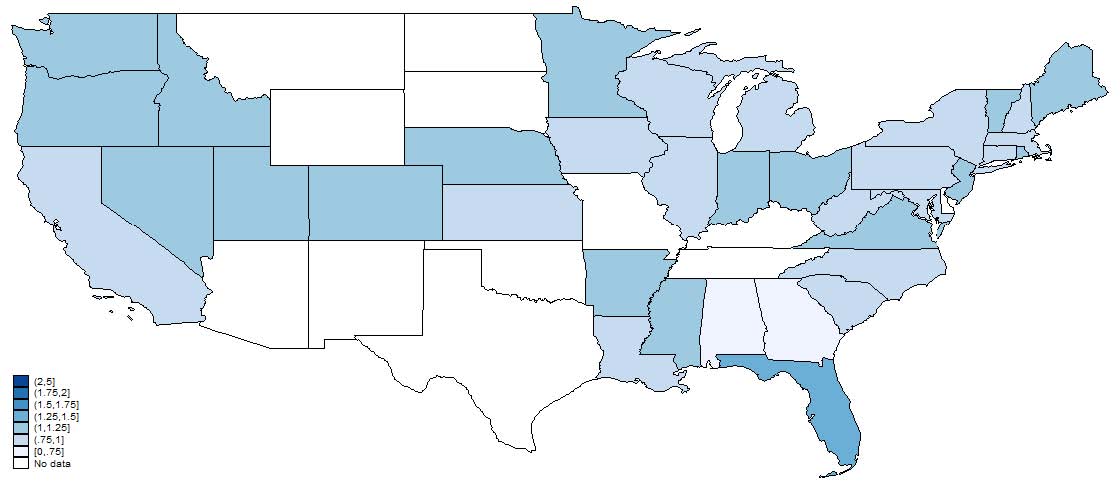
Figures 4, 5, and 6, show the relative representation in patenting by age, gender, and race in 1880, 1910, and 1940. Note that states in white, which represent no data, does not necessarily mean that there were no patentees in that state-year only that we were unable to match anyone. Most striking is the persistence in these state-level representation patterns. States that tend to have high representation of, say, women in 1880 tend to have high representation in 1940. This is suggestive that, at least in a relative sense, state differences are important in explaining demographic differences. We also note that these patterns are not “broadly” geographical in that it is not a purely Southern versus Northern phenomenon nor east versus west coast.
3.5 County-level
We now offer some exploratory regressions to predict the the characteristics of inventors based on characteristics of the county in which they live. We estimate simple linear specifications where we predict overall patenting rates, black inventor, female inventor, and inventor age. Note that these first three dependent variables are binary so we are estimating linear probability models. We cluster the standard errors at the county-level in these OLS regressions. We consider multiple specifications: (1) including no region fixed effects, (2) including just a southern state fixed effect,
(3) including state effects, and (4) for the female and black estimations, an “intensive margin” regression that restricts attention to counties having at least one patent by a woman or African American. By comparing this last specification to the others, we can identify whether these county-characteristics are mainly important for just whether or not a particular group participates at all. Finally, it should be kept in mind that the matched dataset is somewhat sparse at the county-level making some of the estimates rather fragile.
Note that the first four rows of each table of regression results report controls for the demographics of the county that we know already are related to the demographics of inventors. Table 2 shows the results for female patent representation. We find unsurprisingly counties with higher fractions of women tend to have higher representation of female patentees. What is perhaps more interesting is that this elasticity is less than one for one, which would be consistent with a model where differences demographics of patentees are simply reflective of local demographic differences. Turning to the other characteristics of the county, we find that women are less likely to be represented in patenting in counties with larger populations. The religious makeup of the counties do not appear to explain much though there is a positive correlation with the fraction of women in manufacturing employment. This is consistent with inventive activity being driven by hands on experience in the production process.
Similarly, table 3 shows that blacks are more represented in patenting in counties with a greater representation of marginalized populations. Counties that have a higher fraction of blacks and women and a lower fraction of cross-state migrants and urban populations are also the ones to have higher representation of black patenting. Interestingly, the only other factor to influence black patenting rates at the county level is white male illiteracy. Counties with a higher fraction of blacks and illiterate white males are those to have higher rates of black patenting. Similar to female patenting, black patenting at the intensive margin is also more or less determined by the same factors that determine black patenting more broadly. The key difference is that here, being in a more populous county enters negatively.
Finally, table 4 shows that patentees in counties with older populations and a higher fraction of whites and males, are also older. Here the relationship between the county-level average age and that of inventors is only slightly smaller than 1. At the county level these patterns prevail but in addition, we find that higher manufacturing employment and greater Jewish representation result in younger patentees. In sum, counties with better female, minority, manufacturing and Jewish representation also have younger patentees. This is consistent with having lower barriers altogether -diversity, and the dominant presence of a sector that employs skilled workers corresponds to age being less of a limiting factor in engaging in inventive activity.
4 Conclusion
This paper presents two main findings. First, we document an incredible degree of persistence in the demographics of patentees in the US over a seventy year period. Comparing our findings to the literature for blacks and females using more current data suggests that these patterns are continuous with the patterns. For ages, it seems that the recent decline since 2000 in the average of inventors is a return towards the pattern that prevailed for the last half of the 19th century and first half of the 20th with the 20 year between 1980 and 2000 as the outlier. Second, we find that it is very difficult to explain the demographics of patentees at the county-level using observable economic and demographic characteristics beyond the most obvious explanatory variable: the fraction of a particular demographic group in the overall county population.
Our findings suggest systematic barriers to inventing activity for women, blacks, and perhaps younger people. While certainly crucial sources of wasted talent, we have not even addressed one of the most often discussed sources of advantage: wealth and intergenerational links. Consider Bell et al. (2015), who study the intergenerational link between patenting of parents and children in the modern US and find high levels of persistence. Most troubling is the fact that gifted children who grew up in poor families are not able to take part in these creative activities. Or consider Link and Ruhm (2013), who based on a survey of inventors on the MIT Tech Review 100, a list of major innovators, finds a correlation of around 0.25 between father and son patenting. Or consider Celik (2015), who on the basis of surnames found that inventors between 1976 and 2000 who came from richter backgrounds were more likely to patent but those from more educated backgrounds had no similar advantage. But to understand whether these correlations are really evidence of misallocation, it is necessary to understand whether these have been stable across history in the face of large institutional changes such as access to higher education. We plan to address this potential source of misallocation by constructing intergenerational links between fathers and sons to examine the persistence in patenting.9
9
It would also be interesting to compare this intergenerational persistence to those measured for income or occupation historically e.g., Long and Ferrie (2013).
References
Abramitzky, R., L. P. Boustan, and K. Eriksson (2012). Europe’s tired, poor, huddled masses: Self-selection and economic outcomes in the Age of Mass Migration. American Economic Review 102, 1832–1856.
Angrist, J. D. and A. B. Krueger (1992). The effect of age at school entry on educational attainment: an application of instrumental variables with moments from two samples. Journal of the American Statistical Association 87 (418), 328–336.
Ashcraft, C. and A. Breitzman (2007). Who invents it? an analysis of women’s participation in information technology patenting. Technical report, National Center for Women in Information Technology.
Bell, A., R. Chetty, X. Jaravel, N. Petkova, and J. van Reenen (2015). Innovation policy and the lifecycle of inventors. Unpublished, Harvard University.
Bertrand, M., C. Goldin, and L. F. Katz (2010). Dynamics of the gender gap for young professionals in the financial and corporate sectors. American Economic Journal: Applied Economics 2, 228– 255.
Celik, M. (2015). Does the cream always rise to the top? The misallocation of talent in innovation. Unpublished, University of Pennsylvania.
Cook, L. D. (2004). African american inventors data set.
Cook, L. D. (2011). Inventing social capital: Evidence from African American inventors, 1843–1930. Explorations in Economic History 48, 507–518.
Cook, L. D. (2014). Violence and economic growth: Evidence from African American patents, 1870-1940. Journal of Economic Growth 19, 221–257.
Cook, L. D. and C. Kongcharoen (2010). The idea gap in pink and black. NBER Working paper 16331.
Cook, L. D., T. D. Logan, and J. M. Parman (2013). Distinctively black names in the American past. NBER Working Paper 18802.
Ding, W. W., F. Murray, and T. E. Stuart (2006). Gender differences in patenting in the academic life sciences. Science 313, 665–666.
Feigenbaum, J. J. (2015). Automated census record linking: A machine learning approach. Unpublished, Harvard University.
Ferrie, J. P. (1996). A new sample of males linked from the public use microdata sample of the 1850 US federal census of population to the 1860 US federal census manuscript schedules. Historical Methods: A Journal of Quantitative and Interdisciplinary History 29, 141–156.
Foley, C. F. and W. Kerr (2013). Ethnic innovation and U.S. multinational firm activity. Management Science 59, 1529–1544.
Frietsch, R., I. Hallerb, M. Funken-Vrohlingsb, and H. Grupp (2009). Gender-specific patterns in patenting and publishing. Research Policy 38, 590–599.
Hsieh, C.-T., E. Hurst, C. I. Jones, and P. J. Klenow (2013). The allocation of talent and us economic growth. Unpublished, Chicago Booth.
Hunt, J., J.-P. Garant, H. Herman, and D. J. Munroe (2012). Why don’t women patent? IZA Discussion Paper 6886.
Jones, B. F. (2009). The burden of knowledge and the “death of the renaissance man”: Is innovation getting harder? Review of Economic Studies 76, 283–317.
Jones, B. F. (2010). Age and great invention. Review of Economics and Statistics 92, 1–14.
Jung, T. and O. Ejermo (2014). Demographic patterns and trends in patenting: Gender, age, and education of inventors. Technological Forecasting and Social Change 86, 110–124.
Kaiser, J. (2008). Science 322, 834–835.
Kerr, W. and W. Lincoln (2010). The supply side of innovation: H-1B visa reforms and US ethnic invention. Journal of Labor Economics 28, 473–508.
Kerr, W. R. (2008). The ethnic composition of US inventors. HBS Working Paper 08-006.
Kerr, W. R. (2010). The agglomeration of U.S. ethnic inventors. In E. Glaeser (Ed.), Agglomeration Economics. University of Chicago Press.
Khan, B. Z. and K. L. Sokoloff (1993). ”Schemes of Practical Utility”: Entrepreneurship and innovation among ”great inventors” in the United States, 1790-1865. Journal of Economic History 53, 289–307.
Lamoreaux, N. R. and K. L. Sokoloff (2005). The decline of the independent inventor: A Schumpterian story. NBER Working Paper 11654.
Link, A. N. and C. J. Ruhm (2013). Fathers’ patenting behavior and the propensity of offspring to patent: an intergenerational analysis. Journal of Technology Transfer 38, 332–340.
Long, J. and J. Ferrie (2013). Intergenerational occupational mobility in Great Britain and the United States since 1850. American Economic Review 103, 1109–1137.
Perlman, E. (2015). Dense enough to be brilliant: Patents, urbanization, and transportation in Nineteenth Century America. Unpublished, Boston University.
Poirier, A. and N. L. Ziebarth (2014). A simple estimator for merged datasets with non-unique identifiers. Unpublished, University of Iowa.
Schmookler, J. (1957). Inventors past and present. The Review of Economics and Statistics, 39, 321–333.
Sokoloff, K. L. (1988). Inventive activity in early industrial America: Evidence from patent records, 1790-1846. Journal of Economic History 48, 813–850.
Sokoloff, K. L. and B. Z. Khan (1990). The democratization of invention during early industrialization: Evidence from the United States, 1790-1846. Journal of Economic History 50, 363–378.
Steckel, R. and N. L. Ziebarth (2013). A troublesome statistic: Traders and the westward movement of slaves. Journal of Economic History 73, 792–809.
Thursby, J. G. and M. C. Thursby (2005). Gender patterns of research and licensing activity of science and engineering faculty. Journal of Technology Transfer 30, 343–353.
|
Year |
1870 |
1880 |
1900 |
1910 |
1920 |
1930 |
1940 |
|
# Patents in Annual Report |
12,894 |
13,441 |
26,414 |
35,769 |
39,542 |
47,938 |
47,830 |
|
% Parsed |
69.7 |
58.7 |
53.3 |
51.9 |
35.7 |
29.9 |
60.0 |
|
% Match of Parsed |
67.3 |
67.6 |
51.9 |
62.0 |
60.5 |
26.4 |
22.7 |
|
% Matched of Total |
46.9 |
39.7 |
27.6 |
32.1 |
21.6 |
7.9 |
13.6 |
|
% Unique |
80.1 |
82.1 |
50.4 |
82.4 |
79.4 |
55.4 |
57.9 |
|
Average # of Matches |
1.40 |
1.37 |
2.12 |
1.35 |
1.42 |
2.03 |
1.93 |
Table 1: Summary statistics comparing initial sample of patentees, our parsed list, and matched sample.
Female Inventor
(1) (2) (3) (4) (5) (6) (7)
Mean Age Frac Female Frac White Frac State Migrant Log Population Frac Urban Frac Illiterate Frac Manuf (fem) Frac Protestant Frac Jewish
-0.00259 (0.00257)
-0.00221 (0.00339)
-0.00203
(0.00276)
0.387∗∗∗
(0.132)
-0.130∗∗∗
(0.0279)
0.0942∗∗∗
(0.0154)
-0.00929∗∗∗ (0.00343) -0.00267 (0.00346)
0.340∗
(0.184)
-0.112∗∗∗
(0.0372)
0.0884∗∗∗ (0.0165)
-0.0159∗∗∗ (0.00404)
0.0147 (0.0118) 0.000151 (0.00369)
0.251 (0.189)
-0.00759
(0.0501)
0.0892∗∗∗ (0.0166)
-0.0132∗∗∗ (0.00403)
0.0153 (0.0118) -0.00750∗∗ (0.00376)
0.264 (0.177)
0.00613
(0.0552)
-0.0869∗∗∗ (0.0335)
-0.00460 (0.00459)
0.0182 (0.0130) -0.00662 (0.00541)
0.709∗∗∗
(0.234)
-0.128 (0.0808)
0.0164 (0.0513)
0.00747 (0.00737)
0.0275∗
(0.0158)
-0.182
(0.663)
0.204∗
(0.123)
0.00593
(0.0200)
-0.654
(2.024) -0.00935∗∗ (0.00456)
0.156 (0.184)
0.0175 (0.0709)
-0.0966∗∗
(0.0407)
-0.0211∗∗∗ (0.00565)
0.0102 (0.0118)
|
Observations |
78396 |
65788 |
39759 |
39759 |
39759 |
14814 |
36685 |
|
Adjusted R2 |
0.016 |
0.019 |
0.019 |
0.019 |
0.025 |
0.010 |
0.030 |
|
Effects Included |
None |
None |
None |
South |
State |
State |
State |
|
Sample |
Full |
Full |
Full |
Full |
Full |
Full |
Intensive |
Standard errors in parentheses
∗ p < 0.10, ∗∗ p < 0.05, ∗∗∗ p < 0.01
Table 2: County-level Correlates of Gender of Patentees. Female is coded as 1. These are linear probability models. All explanatory variables are from the Population Census. Note that implicitly counties with no patentees are dropped. Standard errors are clustered at the county-level. All regressions include year fixed effects.
Black Inventor
(1) (2) (3) (4) (5) (6) (7)
Mean Age Frac Black Frac Male Frac State Migrant Log Population Frac Urban Frac Manuf Frac Illiterate Frac Illiterate M Frac Illiterate B Frac Protestant Frac Jewish
|
-0.0142∗∗∗ (0.00195) |
-0.00335∗∗∗ (0.00122) |
-0.00296∗∗∗ (0.00111) |
-0.00223∗∗ (0.00107) |
-0.00155 (0.00144) |
|
0.410∗∗∗ (0.0282) |
0.342∗∗∗ (0.0314) |
0.316∗∗∗ (0.0449) |
0.316∗∗∗ (0.0499) |
|
-0.0164 (0.0604) |
-0.107∗∗∗ (0.0399) |
-0.0831∗ (0.0439) |
-0.0736 (0.0657) |
|
-0.0193∗∗∗ (0.00560) |
-0.0159∗∗∗ (0.00480) |
-0.0158∗∗∗ (0.00473) |
-0.0145 (0.0194) |
|
0.00146 (0.00193) |
0.00389∗∗∗ (0.00134) |
0.000853 (0.00102) |
0.00157 (0.00127) |
0.00322∗ (0.00173) |
|
|
-0.00183∗∗∗ (0.000693) |
-0.00171∗∗∗ (0.000658) |
-0.00150∗∗ (0.000694) |
-0.00159 (0.00236)
0.475∗∗∗
(0.180)
0.0601
(0.103)
0.00293
(0.0311)
0.00431 (0.00303)
0.00106 (0.00717)
0.00672
(0.0387)
0.790∗
(0.453)
1.022 (1.584)
-0.577
(0.897)
0.0151 (0.0140)
-1.822∗
(1.000) -0.00984∗∗ (0.00410)
0.367∗∗∗
(0.113)
-0.286∗
(0.153)
-0.0152
(0.0264)
-0.00887∗∗ (0.00388)
-0.0359∗∗
(0.0151)
|
Observations |
58195 |
50276 |
29800 |
29800 |
29800 |
8127 |
17476 |
|
Adjusted R2 |
0.026 |
0.066 |
0.053 |
0.053 |
0.058 |
0.088 |
0.094 |
|
Effects Included |
None |
None |
None |
South |
State |
State |
State |
|
Sample |
Full |
Full |
Full |
Full |
Full |
Full |
Intensive |
Standard errors in parentheses
∗ p < 0.10, ∗∗ p < 0.05, ∗∗∗ p < 0.01
Table 3: County-level Correlates of Race of Patentees. Non-white is coded as a 1 in these regressions. These are linear probability models. All explanatory variables are from the Population Census. Note that implicitly counties with no patentees are dropped. Standard errors are clustered at the county-level. All regressions include year fixed effects.
Age of Inventor
(1) (2) (3) (4) (5) (6)
|
Mean Age |
0.971∗∗∗ (0.0715) |
0.876∗∗∗ (0.0702) |
0.755∗∗∗ (0.0926) |
0.739∗∗∗ (0.103) |
0.729∗∗∗ (0.138) |
0.747∗∗∗ (0.215) |
|
Frac Male |
|
-6.292∗ (3.406) |
-13.75∗∗∗ (4.878) |
-14.25∗∗∗ (5.013) |
-11.24∗ (5.837) |
-21.23∗∗ (10.15) |
|
Frac White |
|
2.704∗∗∗ (0.933) |
2.390∗ (1.251) |
1.840 (1.759) |
1.217 (1.759) |
8.406∗∗ (3.333) |
|
Frac State Migrant |
|
0.728∗ (0.420) |
0.540 (0.500) |
0.539 (0.500) |
-1.718 (1.104) |
0.289 (2.447) |
|
Log Population |
-0.250∗∗∗ (0.0845) |
-0.381∗∗∗ (0.0761) |
-0.251∗ (0.129) |
-0.266∗∗ (0.132) |
-0.151 (0.153) |
0.171 (0.295) |
|
Frac Urban |
|
|
-0.277 (0.454) |
-0.279 (0.454) |
-0.233 (0.395) |
0.617 (0.775) |
|
Frac Manuf |
|
|
|
|
|
-7.764∗∗ (3.888) |
|
Frac Illiterate |
|
|
|
|
|
4.291 (25.34) |
|
Frac Protestant |
|
|
|
|
|
-0.300 (1.109) |
|
Frac Jewish |
|
|
|
|
|
-140.0∗∗ (64.96) |
|
Observations |
58195 |
50276 |
29800 |
29800 |
29800 |
8127 |
|
Adjusted R2 |
0.015 |
0.017 |
0.013 |
0.013 |
0.015 |
0.022 |
|
Effects Included |
None |
None |
None |
South |
State |
State |
|
Sample |
Full |
Full |
Full |
Full |
Full |
Full |
Standard errors in parentheses
∗ p < 0.10, ∗∗ p < 0.05, ∗∗∗ p < 0.01
Table 4: County-level Correlates of Age of Patentees. All explanatory variables are from the Population Census. Note that implicitly counties with no patentees are dropped. Standard errors are clustered at the county-level. All regressions include year fixed effects.

(a) Age (b) Race

(c) Sex (d) Interstate Migrant
Figure 1: Demographics of patentees relative to county of residence. The mean is the average characteristic across all possible matches for a given patentee, then averaged across all patentees. The max (resp. min) is the “maximum” (resp. “minimum”) value of a particular characteristic across all possible matches, then averaged across all inventors. We then report the ratio of these statistics to the average characteristics of the population in the county.

(a) Sex

(b) Race
Figure 2: Fraction of males and black based on first names of patentees. This uses a “2-sample IV” procedure to impute a probability that a particular inventor is male (resp. black) based on the probability that a person with that first name is male (resp. black) in the nearest population census. Note that with this procedure, we can calculate a fraction for each year of the Annual Report of the Patent Commissioner.

(a) Sex

(b) Race
Figure 3: Distribution of ages of inventors by race and sex reported as total patents by particular group (male, white) over total population (multiplied by 10,000).

(a) 1880

-
(b)
-
1910
(c)
1940

Figure 4: Relative age of inventors to the county-level reference population. Note that states with no reported data do not necessarily imply there were no patents in that state but that we were unable to match any inventors from that state. Inventor characteristics are from the best match in the Population Census for a particular inventor.

(a) 1880

-
(b)
-
1910
(c)
1940

Figure 5: Relative frequency of male inventors to the county-level reference population. Note that states with no reported data do not necessarily imply there were no patents in that state but that we were unable to match any inventors from that state. Inventor characteristics are from the best match in the Population Census for a particular inventor.

(a) 1880

-
(b)
-
1910
(c)
1940

Figure 6: Relative frequency of white inventors to the county-level reference population. Note that states with no reported data do not necessarily imply there were no patents in that state but that we were unable to match any inventors from that state. Inventor characteristics are from the best match in the Population Census for a particular inventor.
A Appendix: Quality of Our List of Patent Grantees
Given that we do not successfully extract 100% of the inventors listed on the Annual Reports , it is natural to ask if there are any systematic biases in our subsample. We are particularly worried about difficulties in the original optical character recognition (OCR) process that produced these machine readable texts. Given the algorithmic nature of the procedure, issues with OCR can generate systematic issues in reading, say, “ff” as “v,” a problem with some OCR software. We are able to fix up some of these biases by recoding some common OCR mistakes, for example first names that start with “AV” are almost certainly meant to start with “W.” However, it is conceivable that some systematic errors remain. There are also possible problems stemming from our parser. There are numerous variations in how each patent is reported within a year. This makes it possible that the regular expressions we used to identify the names and locations of patentees are failing to account for all possible variations in how these are recorded.
To check that both of these problems are not driving persistent differences, we compare our parsed dataset to a comprehensive dataset constructed by Jim Shaw and the maintainers of the Directory of American Tool and Machinery Patents, which we refer to below as the “Jim Shaw data.” This dataset was assembled by hand, so it avoids biases inherent in OCR. Unfortunately, the Jim Shaw data usually only records inventors’ first initial, making it mostly unusable for census marching purposes. In addition, the Jim Shaw data only covers the period from 1836 to 1873. Still for four years (1870-1873), our data overlap with Jim Shaw’s, allowing us his as a point of comparisons.
Figure 7 compares the characteristics of patentees including the first letter of first name, first letter of last name, and number of characters in last name for our parsed data and the Jim Shaw data for the years 1870 and 1873. Results for 1871 and 1872 are nearly identical. We plot the relative frequency in our dataset to that of Jim Shaw’s for these characteristics as well as the fraction of patentees that have a particular value for these characteristics. We find that deviations between our sample and Jim Shaw’s only occur, when they do, for characteristics that are quite rare. For example, in panel (c), there are deviations in the relative frequency of length of last name, but these are for very long last names that are exceedingly rare. This gives us some confidence that our sample of patentees to match to the Census does not have systematically different names from the complete population of patentees. Still we note that these results do not imply that the correspondence between our data and Jim Shaw’s for any particular patentee is good only that in the aggregate, possible differences at the patentee level average out.
B Appendix: Matching Procedure
To perform the matching, we use Stata’s reclink command, which is a modified bigram string comparator that returns a “distance” (match score) between two strings. 10 We matched on first name, last name, and town while requiring an exact match on state. The information we are matching on is rather limited relative to other work in the literature which also uses information on age or location of birth (Ferrie, 1996). To aid the matching procedure, for both the list of patentees and census data, we also “regularized” town names from “St.” to “Saint”, removed “District,” “Borough,” and “Ward” from town names as well as removed the “special” characters such as ();,”’ from both datasets. We also used a set of common abbreviations of first names to ensure the consistency of how first names were recorded e.g. “Wm.” became “William.” We removed from the census dataset all individuals less than 15 or more than 80 years old under the assumption that
The same algorithm is also used to match slave traders to shipping manifests (Steckel and Ziebarth, 2013). (a) First Letter of First Name, 1870 (b) First Letter of First Name, 1873


(c) Length of Last Name, 1870 (d) Length of Last Name, 1873

(e) First Letter of Last Name, 1873 (f) First Letter of Last Name, 1870
Figure 7: Comparison of the names of our parsed sample of patentees relative to Jim Shaw sample for 1870, 1871, and 1872. The left hand axis plotted in blue dots shows the relative frequency in our dataset to that in Jim Shaw’s. The right hand axis plotted with yellow bars shows the distribution of Jim Shaw’ data for these various characteristics.
very few of these individuals obtain a patent in any given year.
In determining what is a possible, it is also necessary to specify weights on the match quality of the various matching characteristics as well as a minimum overall match score. To specify these parameters, we compared the matches identified by the algorithm for numerous combinations of matching weights in 1900 Vermont to the set of matches identified by “hand.”11 Vermont is, of course, not the most representative state since it tends to have relatively small towns making it easier to identify patent grantees based solely on name, but it has few enough patentees that it is feasible to check all of them by hand and a large enough number that we can be reasonably confident that matching results are not driven entirely by chance. The best parameters in specifying what is a match are able to match 76.4% (39 of 51) of Vermont patentees. Of the 12 unmatched patentees, we were unable to locate 4 through a manual search of the whole state, 2 returned possible matches at the state level although with wrong town name, and 4 (2 unique individuals, one of whom had 3 patents) more returned possible matches at the county level although again with wrong town name. The remaining two unmatched individuals were found as possible matches in the correct county. There were also 5 “false positive” matches, all of which had intermediate match scores.
A perennial question in this matching literature is the less than perfect match rate. Of course, some of this failure to match people over time is due to deaths or immigration out of the country, but rates still tend to be too low. In our case where in principle we know that someone is living in a particular town, the explanation, at least in part, must be that people move between the time when the patent application is filed and when it is granted. In this case, the location recorded in the patent report that of the location when the application is filed would be incorrect and it would be impossible to locate the patentee in the census records. To address this, we plan to experiment with matching to Annual Reports in years adjacent to the census years. For example, we would match the 1901 or 1902 volume of patent grantees to the 1900 population census. The location recorded is the inventor’s place of residence at the time of patent application and, given the lag in patent approval, matching to 1901 or 1902 patent report to the 1900 census could potentially better reflect where inventors were located in 1900.
As noted in the text, our matching procedure returns any person in the census who is a potential match and does not enforce that matching be “injective.” There are several ways to handle the resulting cases of multiple potential matches, and we experiment with several below. First, we select the “best” match, which is the match with the highest match score; when multiple individuals produce the same match score, we randomly pick one as the best match. Second, we construct best-case and worst-case bounds on statistics of interest using the data on all potential matches. In particular, we calculate, say, the bounds on the average age by taking the average of the maximum and minimum ages of possible matches patentee by patentee. Finally, we average over all possible matches as suggested by Poirier and Ziebarth (2014). This treats all of the possible matches as exchangeable and it hinges on the fact that with probability one, the true match is in the set of possible matches. This provides a reason for having a fairly loose matching criteria (though Poirier and Ziebarth (2014) show the costs in efficiency associated with many possible matches).
This procedure is essentially an informal support vector machine, a technique from the machine learning literature. See Feigenbaum (2015) for some work on this algorithmic matching topic.
(a) First Letter of First Name

1880 1920
1880 1920
1880 1920
:Comparing characteristics of names of matched to non-matched patentees.
(b) First Letter of Last Name

(c) Length of Name
